Kevin Webber

The binary search tree algorithm (BST) is one of the most important algorithms in computer science. Understanding how a binary search tree works is a worthwhile endeavour, as the learnings from BSTs can be applied to more advanced algorithms, or simply be a source of inspiration for your own designs.

In this essay we’ll attempt to fast track learning this important algorithm by visualizing BSTs with GraphStream, a graph diagramming library for Java. Visualizing tree structures may help to accelerate our understanding of their implementation and behaviour.

Hopefully this essay delivers on two fronts:

Providing you with a basic knowledge of GraphStream as an option for visualizing trees and graphs
Providing a better understanding of tree behaviour through visualization techniques

The first section of this essay is my own interpretation of binary search trees from the wonderful book Algorithms 4th Edition by Robert Sedgewick and Kevin Wayne, which I highly encourage reading after this essay. What makes this writing unique is the extra flavour added after completing the optional exercises in the book, which increased my understanding of how BSTs can be leveraged in a variety of problem spaces.

Binary search tree primer

Trees are a fundamental data structure at the heart of many diverse problems we tackle as developers, from product catalogs in e-commerce, to ASTs (abstract syntax trees) in compilers, to how JSON and YAML documents are processed. Whenever faced with a problem best solved by a hierarchical structure, understanding binary search trees might help to inform a solution even if you don’t ever hand code your own BST. This deeper understanding also tees us up for tackling more complex problems represented by graphs, such as routing in shipping & logistics, and relationships in social networks.

Before we get started on how to visualize binary search trees, lets cover some fundamental properties of BSTs and why they make a great candidate for visualizing in order to learn their properties.

A binary tree is made up of nodes. Each node is pointed to by exactly one other node. The only exception is the root node, which has no nodes pointing to it, making it the ancestor of the entire tree. Each node has one child, two children (a full node), or no children (a leaf node). Each child node is a subtree that are themselves considered binary trees.

A binary search tree is an ordered binary tree. A binary tree itself has no special rules or properties aside from what we described above. However, a binary search tree inserts keys in order to make searching the tree more efficient. Keys must be comparable to each other to make this possible.

The basic data structure of a a binary search tree is shown below. It contains a Node type and an instance of a root node, which has a key, a value, up to two children, and a size N which represents the size of the current subtree.

 1    public class BST<Key extends Comparable<Key>, Value> {
 2        private Node root;
 3        private class Node {
 4            private Key key;
 5            private Value value;
 6            private Node left, right;
 7            private int N;
 8            public Node(Key key, Value val, int N) {
 9                this.key = key;
10                this.value = val;
11                this.N = N;
12            }
13        }
14        //TODO (additional code goes here)
15    }

This data structure is not much more complicated than an array or a linked list. The main difference between a binary tree (above) and a linked list is that each node of a binary tree may point to (up to) two children, whereas each node in a linked list can point to one node or no nodes (although a node in a doubly-linked list also points to its parent).

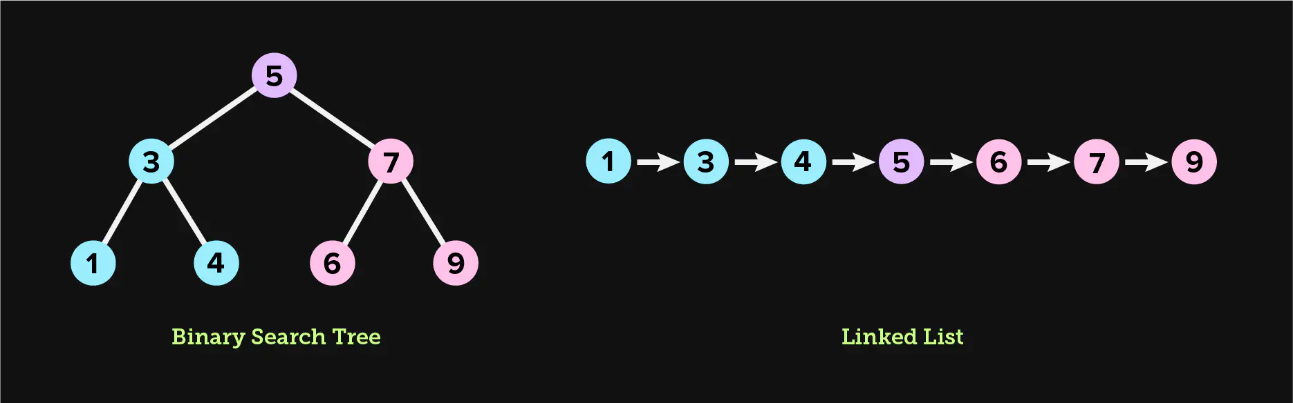
The purpose of a binary search tree is to provide optimal worst case performance for both lookups and inserts. In the example above, looking up 4 takes exactly 3 steps for both the binary search tree and the linked list, as there are 2 edges to navigate, plus 1 step for the root node. However, looking up 9 takes 3 steps in the binary search tree and 7 steps in the linked list, a notable difference that would be even more significant for a larger dataset.

Next, we’ll show exactly how to add nodes to a tree, and discuss the ordering rules that make a binary tree a BST.

Inserting nodes into a binary search tree

In a binary search tree, all keys in the left subtree must be smaller than the key of the current node, and all keys in the right subtree must be larger than the key of the current node.

To insert a new node into the tree, we must traverse down either the left subtree or right subtree to find the correct position to insert a new node into the tree. This means we have to find the first appropriate and empty left child or right child position that meets the criteria we outlined in the above paragraph.

To rephrase the ordering rules, the key for the current node must be larger than all of the keys in the left subtree, and smaller than all of the keys in the right subtree.

 1    public void put(Key key, Value value) {
 2        root = put(root, key, val);
 3    }
 4
 5    private Node put(Node x, Key key, Value value) {
 6        // backtrack and assign the new node to either the left or right
 7        // child of the parent, along with N value of 1 as the new Node
 8        // is a subtree itself
 9        if (x == null) { 
10            return new Node(key, value, 1);
11        }
12        
13        // compare the current node's key to the provided key
14        int cmp = key.compareTo(x.key);
15        
16        // if the provided key is smaller than the current node's key,
17        // we will place the new node somewhere in the left subtree
18        // or assign to x.left if empty
19        if (cmp < 0) {
20            x.left = put(x.left, key, value);
21        }
22        // otherwise, we will place the new node somewhere in the right subtree
23        // or assign to x.right if empty
24        else if (cmp > 0) {
25            x.right = put(x.right, key, value);
26        }
27        // if the provided key matches the current key, we update the value
28        else {
29            x.val = val;
30        }
31
32        // update the size of this subtree to reflect the new node
33        x.N = size(x.left) + size(x.right) + 1;
34
35        return x;
36    }

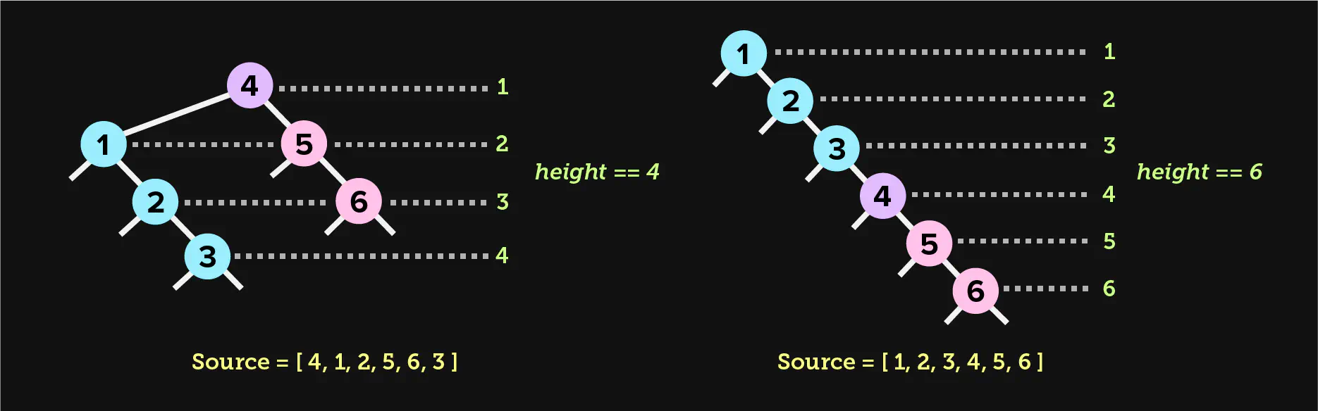
When we call this method with a key and value, our code recursively walks through the tree to determine the correct path, left or right. It may become clear that the height of a binary search tree is completely dependent on the order of the data that we use to pollinate the tree. Binary search trees are ordered but unbalanced. This means that insertion will follow the simple rules we outlined above, but not prevent a single subtree from growing too large. If we use an ordered list to construct a binary search tree, the resulting tree will be suboptimal.

This simple set of rules is what makes a binary tree a binary search tree, which makes it possible to search for a key in worst-case O(h) time, where h is the height of the tree. Therefore, the height of the tree is very important for the efficiency of searching a BST. In a situation where the height of the tree is equal to the size of the original input used to create the tree, the effective worst-case time complexity of lookups will be O(n). This happens if we construct a BST from ordered data. BST construction depends on keys to be inserted in a random order for best performance.

Now that we have the necessary ingredients mixed together for baking a valid binary search tree, we need to add additional functions to make the tree delicious.

Implementing size, rank, and depth functions

Lets discuss three functions that a binary search tree must implement to be generally useful: tree size, node rank, and node depth. These functions are all required in order to visually render a tree, and will be called later in the essay when we demonstrate how to display a tree with GraphStream.

Size

A size function will return the total number of nodes in each subtree, including the root node. Each node will have an x.N value, which represents the size of the subtree. Therefore, the x.N value of the root node is the size of the entire tree.

 1    // Number of nodes in the tree
 2    public int size() { 
 3        return size(root);
 4    }
 5
 6    // Number of nodes in the subtree
 7    private int size(Node n) {
 8        if (x == null) return 0;
 9        else return x.N;
10    }

In a properly implemented BST, each node will maintain a precomputed size of its subtree, which will be kept up-to-date as items are inserted and removed from the tree. The method above returns a precomputed x.N.

If you recall, in our put(...) method, we first assigned a new Node to x.left or x.right (or updated the value if the key existed). We then updated x.N with the new size of the subtree, including the new Node. This is more efficient than recursively computing the size of the tree each time size() is called.

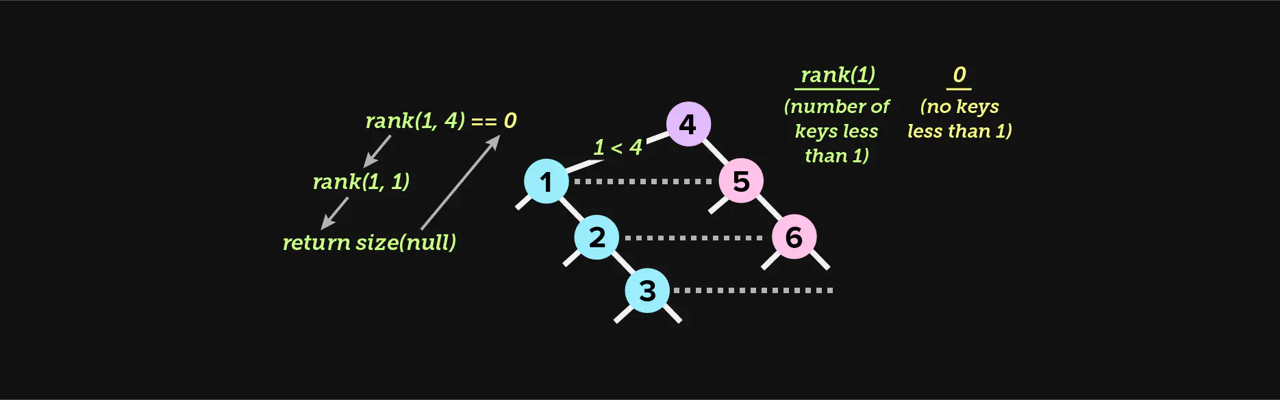
Rank

The rank of a node is the count of all nodes in a tree with a smaller key value than the provided key. For instance, if we flatten a binary search tree and arrive at the following key values of 1, 5, 10, 15, and 20, rank(10) will yield 2. This function is how we will plot a node along the horizontal plane of our diagram later in the essay.

 1    // Number of keys in the tree less than the provided key
 2    public int rank(Key key) {
 3        return rank(key, root);
 4    }
 5
 6    // Number of keys in the subtree less than the provided key
 7    private int rank(Key key, Node x) {
 8        if (x == null) {
 9            return 0;
10        }
11        
12        // compare the current node to the search key
13        int cmp = key.compareTo(x.key);
14        
15        // the match is in the left subtree (if a match exists)
16        if (cmp < 0) { 
17            return rank(key, x.left);
18        }
19        // accumulate the size of the left subtree whenever we begin to search 
20        // the right subtree
21        else if (cmp > 0) { 
22            return 1 + size(x.left) + rank(key, x.right);
23        }
24        // we found a match, so return the size of the left subtree, which may
25        // or may not be accumulated with other subtree counts as we pop up the stack
26        else {
27            return size(x.left);
28        }
29    }

We begin by comparing the key of the current node to the key we’re searching for. If the key we’re searching for is less than the current node’s key, we recursively return the rank of the left subtree. We don’t need to find an exact match so we may run into a null node, in which case we return 0 and accumulate with other return values if any exist (more on accumulators in the next paragraph).

Things become interesting if the key is greater than the key of the current node (lines 21 to 23). This means that the answer must exist in the right subtree. Before we recurse right, we accumulate the size of the left subtree, and any other left subtree that came before. We also add 1 to represent the size of the current node. As recursion unwinds, this line of code will accumulate the size of all left subtrees before the boundary, therefore determining the rank.

We’ve added inline comments to help navigate the above logic, as the accumulator on line 22 might seem unfamiliar unless you have functional programming experience. For more insight into accumulators and folds, this blog post outlines a nice overview in Python, and is also a gentle introduction to functional programming. Once you’re familiar with accumulators and other general approaches to common problems, it becomes easier to port imperative solutions to recursive solutions, and recursive solutions to pure functional solutions.

Depth

Finally, we need to be able to determine the depth of a given node, which is the count of edges from a given node to the root node. Edges will be covered in greater detail when we display our graph.

 1    public int depth(Key key) { 
 2        return depth(key, root, 1); 
 3    }
 4
 5    private int depth(Key key, Node x, int level) { 
 6        // we reached an empty node, backtrack with 0
 7        if (x == null) return 0; 
 8
 9        // we found a match, backtrack with the level
10        if (x.key == key) return level;
11
12        // traverse all the way left until a match is found or we hit an
13        // empty node
14        int leftLevel = depth(key, x.left, level+1);
15        
16        // if we found a match in the left subtree, return it
17        if (leftLevel > 0) {
18            return leftLevel;
19        } 
20        // no match is to be found in the left subtree, search right and repeat
21        // the above steps
22        else {
23            return depth(key, x.right, level+1);
24        }
25    }

This is another example of depth first traversal. If the matching key is found in the left subtree, the level of the key is returned, which has been incremeted with each recursive call. If the key is not found in the left subtree, the match must be in the right subtree if a match exists. Eventually the function backtracks when either a match is found or all nodes have been visited, in which case no match is found and 0 percolates all the way up the stack as the final result. If a matching key is found, the level value is returned.

With these few methods we’ve already implemented, we can construct a basic BST, populate it with data, and be ready to visualize it with very little code remaining to complete!

Pollinating a sample BST with data

Our final step before visualizing the BST with GraphStream is to pollinate our “MVT” (minimum viable tree) with some sample data. In order to do this, we need to implement a method that calls the constructor of our BST. Let’s create a main(...) method.

 1    public static void main(String[] args) {
 2        BinarySearchTree<Integer, Integer> bst =
 3            new BinarySearchTree<Integer, Integer>();
 4
 5        Random generator = new Random();
 6        for (int i = 0; i < 49; i++ {
 7            int rando = generator.nextInt(1000);
 8            bst.put(new Integer(rando), new Integer(i));
 9        }
10
11        // TODO (additional code here)
12    }

The above code creates a BST with random sample data. As our BST is an abstract data type (ADT), we’ve typed the tree with <Integer, Integer>, meaning that our tree can accept an integer in the Key position and an integer in the Value position.

In production code we want to take advantage of Java’s rich type system rather than use primitive wrappers. For instance, if we’re using a BST to store a company directory, we may type our BST with <EmployeeID, Employee>.

This isn’t a very useful BST implementation (yet) as we can’t do anything interesting, like search for a key, but it does give us a chance to implement a few additional functions:

Validate if the BST is correctly formed
Print the structure of the BST

Let’s implement the basic amount of code required to validate that we implemented a correct BST. This will give us yet another opportunity to traverse a BST. There are a number of ways to traverse a tree in order to search for a node or print the contents, which we will discuss in a little more detail.

Validating a BST

In order to validate a tree, we must traverse it. There are many other approaches to traversing a tree. The two main categories of traversal are depth first and breadth first:

Depth first means that we begin from the root node and then visit all nodes in one branch until we reach the bottom of a branch before backtracking, then move laterally and repeat, until we visit all nodes in the tree
Breadth first means we visit all nodes at our current depth before sinking one level lower, and visiting all of the nodes at that depth, and so on, until we visit all nodes in the tree

We will only cover depth first traversal in this essay. Specifically, depth first traversal can be divided into three types:

Depth first, inorder traversal (left, root, right)
Depth first, preorder traversal (root, left, right)
Depth first, postorder traversal (left, right, root)

As a refresher, a BST is a tree with the following properties:

Each node has a Key and a Value
Keys are Comparable
The key of the current code is larger than the keys of the entire left subtree, and the key of the current node is smaller than the keys of the entire right subtree

With that in mind, let’s write some validation code!

 1    public boolean isValidBST() {
 2        return validate(root, null, null);
 3    }
 4
 5    private boolean validate(Node x, Key min, Key max) {
 6        // our goal is to visit every null child in the tree
 7        // therefore, this is our base case
 8        if (x == null) return true;
 9
10        // ensure that the current node is within min/max bounds
11        if ((min == null || x.key.compareTo(min) > 0 &&
12                (max == null || x.key.compareTo(max) < 0)) {
13            
14            // check if the left child is in order
15            if (x.left != null &&
16                    x.left.key.compareTo(x.key) >= 0) {
17                return false;
18            }
19
20            // check if the right child is in order
21            if (x.right != null && 
22                    x.right.key.compareTo(x.key) <= 0) {
23                return false;
24            }
25            
26            // traverse inorder, left then right
27            return validate(x.left, min, x.key) &&
28                validate(x.right, x.key, max);
29        }
30
31        // failed the min/max check
32        return false;
33    }

The above traversal is another example of depth first inorder search; left, root, right. This is most evident by inspecting line 21 and 22. Line 21 will continue to be called until we reach the deepest leftmost node. Then we backtrack, and then we finally traverse right, eventually backtracking all the way with true or short circuiting with false. The BST is valid if lines 21 and 22 never short circuit. In other words, our base case is the null check on line 6. The point of recursion in the happy path is that we reach line 6 for every null child and return true. If we’re unable to visit every null child in the tree, that means the tree is invalid as the conditional logic short circuited and prevented our visit.

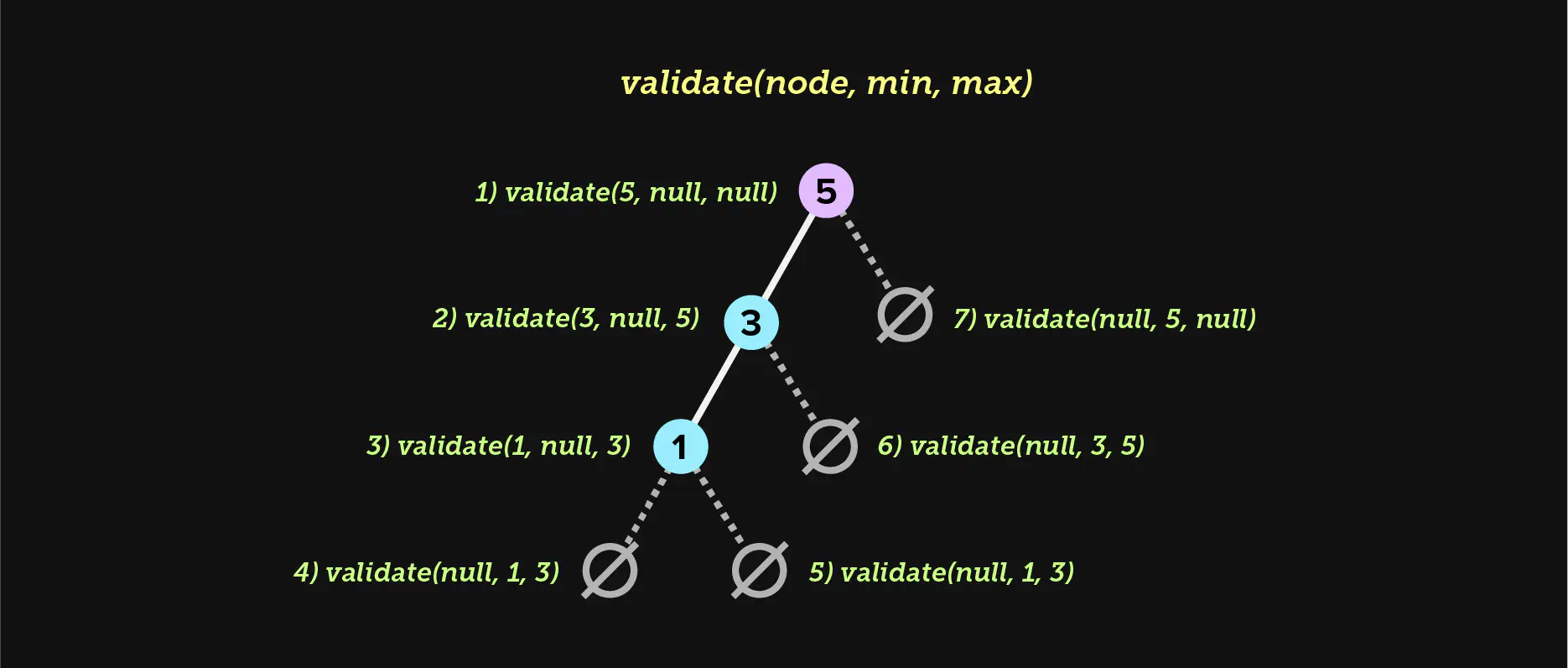
We need to keep track of two boundaries, min and max. When we traverse left, we use the current node’s key as the new max for the next left subtree we visit. When we traverse right, we use the current node’s key as the new min for the next right subtree we visit. This essentially creates a fence, and all keys must remain within that fence. If the current node is ever larger than the max or smaller than the min (lines 8 and 9), we stop recursion and backtrack with false. Because lines 21 and 22 use the && short circuit operator, false percolates all the way up. If we successfully visit all empty nodes without short circuiting, the tree is valid.

(If the root node is null, we return true immediately, as a BST is valid when empty.)

Printing the tree

Now that we’ve learned how to implement core BST algorithms like put(...) and validate(...), we’re ready to print our tree using GraphStream. Before we get started, let’s first cover basic GraphStream semantics.

GraphStream is based on a layout system anchored by x,y coordinates. The contents of our graph can either be completely fluid and layed out automatically, or fixed in place and layed out manually. If we were diagramming a flexible structure, perhaps particle interactions or some other type of physical system, a fluid coordinate system (no pun intended) might be appropriate. In this case we don’t wish for users to be able to drag nodes around the screen, so we’ll take advantage of GraphStream’s ability to style a diagram with CSS and fix the x,y coordinates in place.

Before we start writing code, let’s pull in the dependencies we need to use GraphStream in our project, gs-core and gs-ui-swing. In this example we’ll use Maven, but you can use any build tool you enjoy. The following code brings in the core GraphStream library along with the Swing UI rendering engine: https://github.com/graphstream/gs-ui-swing.

GraphStream also provides Android and JavaFX viewers. It’s also possible to implement customs viewers. For the purposes of this tutorial the Swing viewer is a perfectly simple choice to use.

 1    <dependency>
 2        <groupId>org.graphstream</groupId>
 3        <artifactId>gs-core</artifactId>
 4        <version>2.0</version>
 5    </dependency>
 6    <!-- https://mvnrepository.com/artifact/org.graphstream/gs-ui-swing -->
 7    <dependency>
 8        <groupId>org.graphstream</groupId>
 9        <artifactId>gs-ui-swing</artifactId>
10        <version>2.0</version>
11    </dependency>

Let’s now set up our basic stylesheet for printing a graph. You’ll quickly learn how flexible GraphStream is! The following code sets up our graph’s style based on the stylesheet we define, which is (mostly) standard CSS. This code also lets GraphStream know that we’ll be using the Swing UI rendering engine. GraphStream is very flexible in the way that it can be styled, so for someone more visually inclined, it’s an excellent way to visualize complex interactive data structures.

 1    public void print() {
 2        String styleSheet =
 3            "node {" +
 4            "	text-alignment: right;" +
 5            "	text-offset: 10px, 0px;" +
 6            "   size: 5px, 5px;" +
 7            "}" +
 8            "node.marked {" +
 9            "	fill-color: red;" +
10            "}";
11
12        System.setProperty("org.graphstream.ui", "swing");
13        Graph graph = new SingleGraph("Binary Search Tree");
14        graph.setAttribute("ui.stylesheet", styleSheet);
15
16        print(root, graph);
17
18        Viewer viewer = graph.display();
19        viewer.disableAutoLayout();
20    }

The core of our logic is on line 16, the print(...) method, which plots each node on the x,y axis and also connects the edge of each node based on parent/child relationships.

We haven’t yet talked about edges. An edge represents the relationship between nodes. The BST we created represents edges through code, specifically the left and right parent/child relationship between nodes. Now we need to represent these relationships visually. In GraphStream, this is as simple as invoking graph.addEdge(...) with the correct parameters, which we will discuss in the next section.

Finally, on line 18 we render and display the graph. Line 19 disables the ability for users to click and drag nodes around. This ensures that the tree stays properly formatted based on the algorithmic rules of binary search trees, which we control with x,y coordinates and our CSS stylesheet.

Plotting nodes and connecting edges

This function is responsible for plotting each node on the correct x,y axis, and then connecting the edges of each node based on their parent/child relationships.

The following is a recursive function that visits the left and right subtree of each node until all nodes have been visited and plotted on the graph. Let’s review the code and then discuss specific operations.

 1    private void print(Node x, Graph graph) {
 2        if (x == null) return;
 3
 4        org.graphstream.graph.Node n = graph.addNode(x.key.toString()); 
 5
 6        // print keys as labels if the graph is reasonably small
 7        if (size() <= 50) {
 8            n.setAttribute("ui.label", n.getId()); 
 9        }
10
11        // plot the depth and rank as x,y coordinates
12        n.setAttribute("x", rank(x.key));
13        n.setAttribute("y", depth(x.key)*-1);
14
15        // visit left and right subtrees
16        print(x.left, graph);
17        print(x.right, graph);
18
19        // add edge from this node to left child
20        if (x.left != null) {
21            String leftKey = x.left.key.toString();
22            graph.addEdge(keyStr + leftKey, keyStr, leftKey);
23        }
24
25        // add edge from this node to right child
26        if (x.right != null) {
27            String rightKey = x.right.key.toString();
28            graph.addEdge(keyStr + rightKey, keyStr, rightKey);
29        }
30    }

We begin by plotting each node on a unique x axis based on the rank(...) of the current key. We then use the depth(...) value to plot the node on the y axis, and multiply by -1 to invert the axis. This is because GraphStream considers 0,0 the middle of the graph and 0,-1 to be one level lower.

In theory, as long as the edges of all nodes are properly connected, its not important that each node be laterally placed on a unique x axis. However, to more clearly visualize a binary tree, it can be helpful to ensure that smaller nodes do not overlap larger nodes horizontally and vice-versa, even if the edges are properly connected.

We finally connect the edges of each node to its left and right children, if they exist (lines 19 to 29).

Rendering a binary search tree

This concludes our whirlwind tour of binary search trees, which we will wrap up with the PNG output of all our hard work. The following graph is easy stylable using stylesheets, so download the code and be creative! If you come up with a wonderful stylesheet, please get in touch and share your work, I’d love to see it.

The final step is to compile and execute our code. Assuming you have Maven configured correctly, this should be as easy as the following.

1    mvn compile
2    mvn exec:java -Dexec.mainClass="Main"

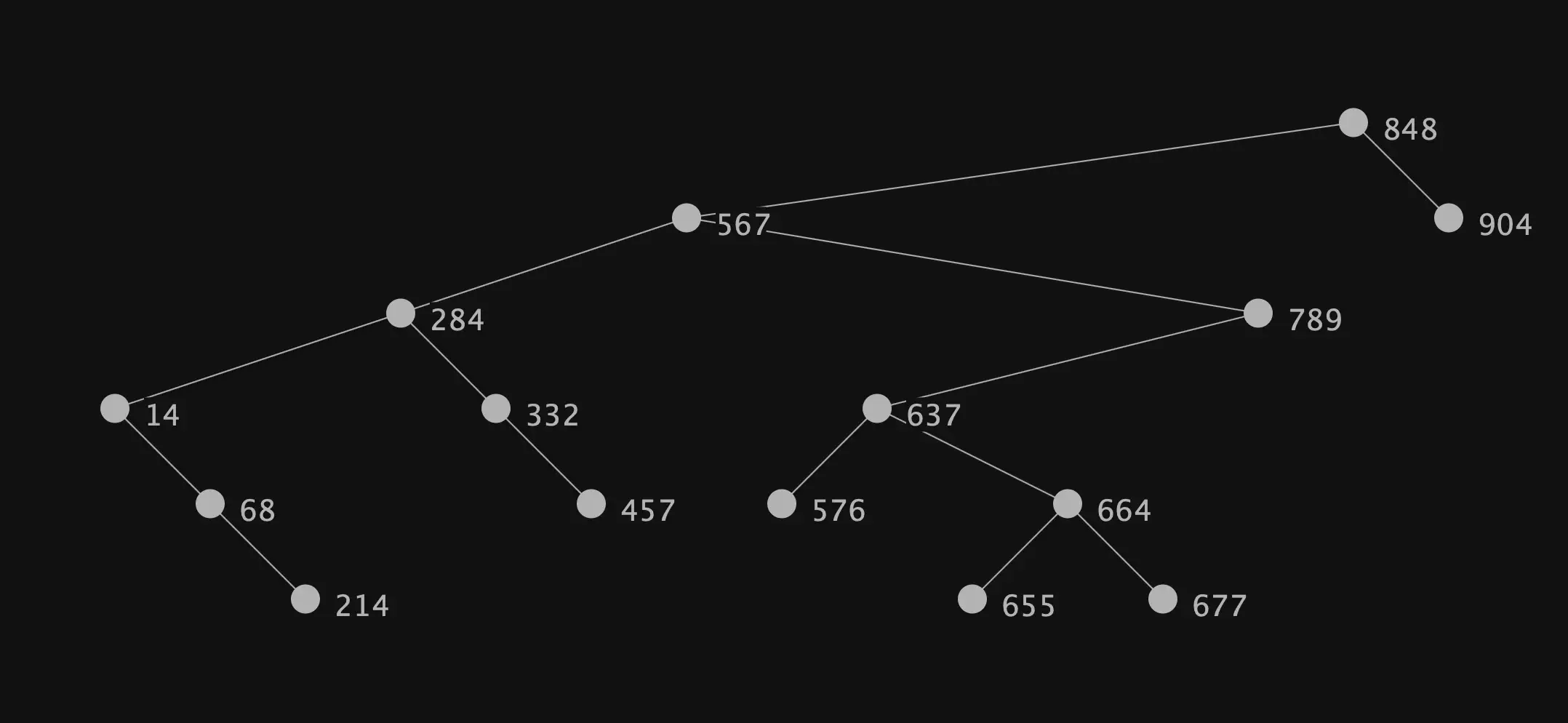
The result is a fully stylable diagram of a binary search tree, developed completely in Java. GraphStream has many other capabilities, including rich UI customization options for building fully featured user interfaces, and even the ability to export movies of animated graphs. The possibilities are endless!

I hope you’ve enjoyed this essay and have discovered a few new tools and techniques that may help to inspire a creative solution for your next project. In the process of writing this essay I’ve developed a deeper appreciation for the elegance of binary search trees and the foundational knowledge that learning and visualizing them has provided.

Visualizing binary search trees with GraphStream